Errors, significant figures and straight-line graphs
Systematic and random errors, fractional and percentage error, significant figures, and turning a relation into a straight line to find a constant.
Kinds of error
Every measurement has some uncertainty. Its causes fall into two kinds.
| Systematic error | Random error | |
|---|---|---|
| Effect | every reading too large (or too small) by about the same amount | readings scatter above and below the true value |
| Examples | zero error, a stretched tape, a slow stop-watch, parallax from always looking at an angle | reaction time when starting a stop-watch, judging a coincidence, small fluctuations |
| Reduced by | correcting the zero error, calibrating, changing method | repeating and averaging, plotting a graph |
Accuracy is how close a result is to the true value (spoiled by systematic error). Precision is how close repeated readings are to each other (spoiled by random error).
Absolute, fractional and percentage error
If a length is $l = 50.0 \pm 0.1\ \text{cm}$, the absolute error is $\Delta l = 0.1\ \text{cm}$. Then: $$\text{fractional error} = \frac{\Delta l}{l} = \frac{0.1}{50.0} = 0.002, \qquad \text{percentage error} = 0.2%$$ Combining errors in a calculated quantity:
- Sum or difference, $y = a \pm b$: add the absolute errors, $\Delta y = \Delta a + \Delta b$.
- Product or quotient with powers, $y = k\dfrac{a^p b^q}{c^r}$: add the fractional errors times the powers, $$\frac{\Delta y}{y} = p\frac{\Delta a}{a} + q\frac{\Delta b}{b} + r\frac{\Delta c}{c}$$
Example: The diameter of a wire is $0.50 \pm 0.01\ \text{mm}$. The area $A = \dfrac{\pi d^2}{4}$ has fractional error $2 \times \dfrac{0.01}{0.50} = 0.04$, which is $4%$. The squared quantity doubles its error. This is why the diameter is measured with a micrometer at several places.
Tip: To reduce the percentage error of a small quantity, measure many of them together. Time $20$ oscillations: a $0.2\ \text{s}$ reaction error on $30\ \text{s}$ is under $1%$, but on one $1.5\ \text{s}$ swing it would be over $13%$.
Significant figures
- All non-zero digits are significant. Zeros between them are significant ($1.05$ has 3).
- Leading zeros are not significant ($0.0042$ has 2).
- Trailing zeros after a decimal point are significant ($2.50$ has 3).
- Use standard form to be clear: $6.52 \times 10^{4}$ has 3 significant figures.
A calculated answer should have no more significant figures than the least precise measurement used. Round only at the end.
Straight-line graphs
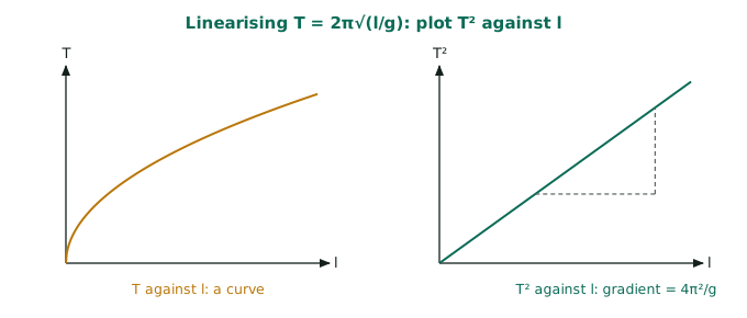
A straight line $y = mx + c$ lets you find constants from the gradient $m$ and the intercept $c$. A graph also averages out random errors and shows up a bad reading. Rearrange the relation so the quantity you vary is $x$ and the quantity you measure is $y$.
| Relation | Plot | Gradient | Intercept |
|---|---|---|---|
| $T = 2\pi\sqrt{\dfrac{l}{g}}$ | $T^2$ against $l$ | $\dfrac{4\pi^2}{g}$ | $0$ |
| $\dfrac{1}{v} + \dfrac{1}{u} = \dfrac{1}{f}$ (real-is-positive) | $\dfrac{1}{v}$ against $\dfrac{1}{u}$ | $-1$ | $\dfrac{1}{f}$ |
| $V = E - Ir$ | $V$ against $I$ | $-r$ | $E$ |
| $N = N_0 e^{-\lambda t}$ | $\ln N$ against $t$ | $-\lambda$ | $\ln N_0$ |
| $T = 2\pi\sqrt{\dfrac{l + d}{g}}$ ($d$ unknown) | $T^2$ against $l$ | $\dfrac{4\pi^2}{g}$ | $\dfrac{4\pi^2 d}{g}$ |
Example: A pendulum gives a $T^2$ against $l$ line of gradient $4.0\ \text{s}^2,\text{m}^{-1}$. Then $g = \dfrac{4\pi^2}{4.0} \approx \dfrac{40}{4.0} = 10\ \text{m s}^{-2}$ (taking $\pi^2 \approx 10$, as the papers often allow).
Exam tip: When asked to "rearrange to obtain a straight-line graph", write the equation in the form $y = mx + c$ and name $y$, $x$, the gradient and the intercept separately. Each usually carries a mark.
When you draw the graph, choose scales that use more than half the grid. Mark points with small crosses. Draw the best straight line, not a dot-to-dot line. Find the gradient from a large triangle, not from two of the readings.